This chapter has been excerpted from the book "Flow-Based Programming: A New Approach to Application Development" (van Nostrand Reinhold, 1994), by J.Paul Morrison. A second edition (2010) is now available from CreateSpace eStore and Amazon.com. The 2nd edition is also available in e-book format from Kindle (Kindle format) and Lulu (epub format). To find out more about FBP, click on FBP.
For definitions of FBP terms, see Glossary.
|
Material from book starts here:
All of the network shapes we have encountered so far have been of the kind we call "batch", and have generally had a left-to-right flow, with IPs being created on the lefthand side and disposed of on the right of the network. Sometimes we need to use a different kind of topology, which is a loop-type network. Several of the later chapters contain examples of this topology, so it is worthwhile spending some time talking about this type of network at a general level. Many networks will in fact be a mixture of the two types, but, once you understand the underlying principles, they won't present any problems.
Here is a very simple example of a loop-type network:
Figure 14.1
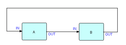
The first question we need to answer about this type of network is: how does it get started? You may remember that the only processes which get started automatically are those with no input connections (IIPs don't count). If you look at Figure 14.1, you will see that there are no processes which have no input connections [double negative intended!]! B has an input connection coming from A, but A has an input connection coming from B! Although on occasion we have been tempted to relax the restriction about which processes can start, the simplest thing to do is just to add an extra process which has no input connections and then use it to start A or B. So the picture now looks like this:
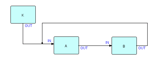
Figure 14.2
where K is the starter ("kicker") process, that emits a single packet containing a blank. K can be connected to either A or B as the logic demands.
Now we have started our loop-type networks, not surprisingly, there is another problem: how do they close down? The problem here is in the definition of close-down of a process - a process closes down on the next deactivation after all of its upstream processes have closed down. In the above diagram, since A is upstream of B, but B is also upstream of A, we get a "catch-22" situation: A cannot close down because B cannot close down until A closes down, and so on. The solution is to provide a special service which makes a process look to its neighbours as if it has closed down. One of the processes involved must then decide to close down and will use this service to notify the other processes. In the batch situation, closedown of the network as a whole was typically initiated by readers closing down (because they had finished reading their files or had run into problems). In loop-type networks, one of the processes - usually one which is interacting with a user - has to decide that no more data is going to arrive, so it closes down.
The service which tells a process's neighbours that it has closed down is one we have mentioned casually before: "close port". FBP lets a component close an input port or close an output port. The function of this service is to close ports before they would normally be closed (this would normally happen automatically at process close-down time, but there are cases, like this one, where we just can't wait that long). A process closing an output port has the same effect on its downstream processes as if the process had terminated. A process closing an input port has the same effect on its upstream processes; also if all of its input ports are now closed, it automatically terminates.
So, to close down the network, A or B in Figure 14.2 simply closes its input or output port - it doesn't matter which one. Suppose B closes its input port and ends execution: it will now terminate [because no more input data can now arrive]. B is in fact A's upstream process, so A will also be able to close down, thus bringing down the whole network (the "kicker" process will have closed down long ago).
Now that we know how to make loop-type networks start and stop, why would we want to use them? This usually has to do with synchronization, which we will also be talking about in a later chapter. In a regular left-to-right network, the left side of the network will be processing the last IPs, while earlier IPs are being processed further to the right in the network. This asynchronism gives this technique a lot of its power, but there are situations where you have to coordinate some processing with a specific external event, or make sure that two functions cannot overlap in time. One such example is that of an interactive application supporting one user. Here A in the above example might be an interactive I/O component and B might be a component to handle the input and generate the appropriate output, e.g.:
Figure 14.3
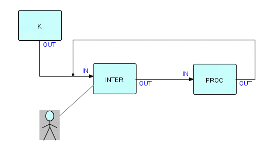
where INTER controls a screen. In this figure, INTER receives some data from PROC, displays it on the screen, waits for some action on the part of the end user, and then sends information back to PROC. If the software infrastructure allows it, waiting for input need only suspend INTER, and other processes could be working on their input while INTER is suspended.
If, on the other hand, this were a left-to-right flow, and PROC were preceded by an input process and followed by an output process (without the "back flow"), input and output to and from the same screen would no longer be synchronized. You therefore have to synchronize at least one component to the pace of the user, so that he or she can act on the data presented on a screen before getting the next screen.
Since the IPs from which a screen is built must fit into the queues of the loop or/and the working storage of the processes, we have to make sure there is enough capacity in these queues. One way to make sure we don't have to worry is to use the tree structures described in an earlier chapter. A tree of IPs can be used to represent the screen data and can be sent around the loop as a unit. Alternatively, the screen data can be represented as one or more substreams, and then we just have to make sure the total queue capacity is set high enough.
As we shall see in Chapter 19, where we describe IBM's IMS on-line applications, you also get a loop structure there, but with a different purpose. IMS is a queue-driven on-line environment, and its Message-Processing Programs (MPPs) keep obtaining transactions from the IMS message queue until there are no more for that MPP, or until certain other conditions are met which cause the MPP to close down. Each time a transaction is obtained from the queue, IMS takes a syncpoint, so any positioning information from the previous transaction is lost, data bases are updated, etc. In FBP, we therefore build MPPs as loops where the next transaction is not read from the message queue until the previous one has been fully processed. The diagram would be the same as the previous one, except that INTER is replaced by a "transaction getter", as follows:
Figure 14.4
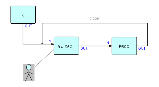
If you are familiar with IMS, you will also realize that each time around this loop the program will normally be dealing with different users, so, unlike the previous example, you cannot use the working storage of the processes to save information relating to one user.
Obviously in both of the above cases, PROC is shorthand for
a
group of processes which collectively process one screenful or
transaction.
This group of processes will accept data from the screen, and send out
some kind of signal when they have finished with it. In both cases, it
doesn't really matter whether the screen output data is routed back to
INTER or GETXACT, or put out by a different process, as
long
as no more input is accepted until the output has been presented to the
user.
[Some paragraphs on subnets and substream sensitivity - including
Figure 14.5 - have been dropped as they are described in more detail in
Chapters 7 and 20.]
Another use for loop networks is for "explosion" applications, of which the classical example is the Bill of Materials explosion, where components of some complex assembly will be "exploded" into subcomponents progressively until they reach ones which cannot be broken down any further. If you know that the largest possible explosion would not fill up storage, you could use a loop of two or more processes with very high capacity queues connecting them (it is dangerous to use a loop with only one process as you could land up getting deadlocked). Of course, the IPs for composite parts must be removed from the data stream when their subcomponents are added to it, or when they are found not to be further reducible (like nuts and screws), so eventually the looping data stream will go empty.
This type of logic can also be useful when parsing other kinds of recursive structures, e.g. lists of lists or expressions in a language. A colleague, Charles Douglas, used it very effectively in a text processing application, where the user needed to be able to name lists of data bases and in turn use those names in other lists. He implemented this very similarly to a Bill of Materials explosion. His application went through all the lists, progressively exploding them until it got down to the actual data base level. Thus suppose, we have the following lists:
A:  B, C, D, E

B:  D, E, G

D:  E, F

Figure 14.6
Then, if you feed in A, the successive stages of explosion are as follows:
A

B, C, D, E

D, E, G, C, E, F, E

E, F, E, G, C, E, F, E

Figure 14.7
If the goal is to figure out how many of each atomic object you have, the totals are:
1 C, 4 E, 2 F, 1 G

Figure 14.8
If you simply want to list the different atomic objects involved, then you get:
C, E, F, G

Figure 14.9
Either way, the simplest technique is to follow the explosion with a Sort, and then either count items, or eliminate duplicates.